Spatio-temporal Interaction Analysis on New York City Shooting Incidents
GEO 511 Spatial Data Science Final Project
Fan Li
Introduction
There are hundreds of shooting incidents in New York city on a yearly basis. Despite the statistics of crime events have been declining since 1990 in New York, in the number of shooting incidents was nearly double in 2020 compared to the year before. Even under the circumstances of COVID-19 pandemic, shooting incidents are still happening by a great number. This project explores the following questions: Are these shooting incidents have spatial and temporal connections? Do they happen in particular regions and time periods? What do the spatiotemporal interaction of these events suggests? And why are they clustered spatially and temporally? What could be done given this spatiotemporal interaction? Some basic hypotheses are: There is spatiotemporal interaction among a part of shooting incidents that happen in New York city every year and they could be explained by socioeconomic factors. The spatiotemporal interaction is tested with a statistical method called Knox statistic test. The correlation of spatiotemporal clusters of shooting incidents and socioeconomic variables are calculated to find causalities. As for results and conclusions, there is spatiotemporal interaction among NYC shooting incidents, and these spatiotemporal clusters have causality relationship with socioeconomic environments.
Key words: Shooting incident, NYC, spatiotemporal interaction, Knox test, socioeconomic factors
Materials and methods
This project employs two datasets, the zip code shapefile of New York city and the 2021 shooting incident data of New York city. Both datasets were downloaded from New York city open data(https://opendata.cityofnewyork.us/). The zip code shapefile contains 263 features identifying different zip codes in New York city. Each feature is tagged with the county name that they belong to. The shooting incident data is in CSV format, it contains the longitude and latitude coordinate of each incident. With these geographic coordinates, it is possible to convert the data frame generated directly from reading CSV file to a Spatial Point Data Frame. After projection, the distance matrix of the incidents could be calculated. These provides conditions to perform Knox statistical test with an R package called surveillance. The R package named surveillance is specialized in temporal and spatio-temporal modeling and monitoring of epidemic phenomena. With Knox test conclude with rejecting null hypothesis of no spatiotemporal interaction, visualization of the count of clustered incidents in each zip code could be produced. Finally, the choropleth map of count of clustered incidents will be compared to a map of median income map by zip codes of New York city. Though the two maps have some differences in partition of the city by zip code, they are basically similar to each other.
library(lubridate)
library(sp)
library(surveillance)
library(mapproj)
library(sf)
library(mapview)
library(GISTools)
library(rgdal)
library(tidyverse)
library(rgeos)
library(lpSolveAPI)
library(dplyr)
library(tbart)Data cleaning and first figure
# Read data
data_y2d <- read.csv("data/NYPD_Shooting_Incident_Data__Year_To_Date_.csv")
zipcode <- as(st_read("data/ZIP_CODE_040114/ZIP_CODE_040114.shp"), "Spatial")## Reading layer `ZIP_CODE_040114' from data source
## `/__w/2021_project-FanLukeLi/2021_project-FanLukeLi/data/ZIP_CODE_040114/ZIP_CODE_040114.shp'
## using driver `ESRI Shapefile'
## Simple feature collection with 263 features and 12 fields
## Geometry type: POLYGON
## Dimension: XY
## Bounding box: xmin: 913129 ymin: 120020.9 xmax: 1067494 ymax: 272710.9
## Projected CRS: NAD83 / New York Long Island (ftUS)# Visualize original data
coordinates(data_y2d) <- ~ Longitude + Latitude
proj4string(data_y2d) <- CRS("+init=epsg:4326")
coords <- data.frame(spTransform(data_y2d, CRS("+init=epsg:2263")))
# data_y2d is a spatial data frame now, visualizing the original datasets is possible
mapview(data_y2d, xcol = "Longitude", ycol = "Latitude", crs = "+init=epsg:2263") +
mapview(zipcode)# Knox test
date <- as.Date(data_y2d$OCCUR_DATE, format = "%m/%d/%y")
startdate <- as.Date("01/01/2021", "%d/%m/%y")
date_number <- difftime(date, startdate, units = "days")
date_numeric <- as.data.frame(as.numeric(date_number))
dt_mat <- dist(date_numeric, diag = TRUE, upper = FALSE)
coords_lonlat <- data.frame(coords$Longitude, coords$Latitude)
dist_mat <- dist(coords_lonlat, method = "euclidean", diag = TRUE, upper = FALSE)
k_test <- knox(dt = dt_mat, ds = dist_mat, eps.t = 3, eps.s = 10)## .......................................................................................................................................................................................................................................................................................................................................................................................................................................................................................................................................................................................................................................................................................................................................................................................................................................................................................................................................................................................................................................# Plot k_test result
# plot(k_test)# Visualize spatiotemporal clusters
c1 <- which(dist_mat <= 10)
c2 <- which(dt_mat <= 3)
c <- intersect(c1, c2)
index_cluster <- c(1:902)
index_cluster <- index_cluster - index_cluster
i <- 0
for (n in 2:902){
for (m in 1:(n-1)){
i <- i + 1;
if (i %in% c){
index_cluster[n] <- 1;
index_cluster[m] <- 1;
}
}
}
data_y2d$CLUSTERED <- index_cluster
# mapView(data_y2d, xcol = "Longitude", ycol = "Latitude", zcol = "CLUSTERED", crs = "+init=epsg:2263") +
# mapview(zipcode)# Generate statistics of spatiotemporal clusters
names(data_y2d)[1] <- "INCIDENT_KEY"
data_y2d_transform <- spTransform(data_y2d, zipcode@proj4string)
data_y2d_transform <- st_as_sf(data_y2d_transform)
clustered_incidents <- data_y2d_transform %>% filter(CLUSTERED == 1)
clustered_incidents <- as(clustered_incidents, "Spatial")
clustered_incidents <- spTransform(clustered_incidents, zipcode@proj4string)
overlay <- clustered_incidents %over% zipcode
zipcode$COUNT <- c(1:nrow(zipcode))
zipcode$COUNT <- zipcode$COUNT - zipcode$COUNT
for (i in c(1:nrow(zipcode))){
zipcode$COUNT[i] <- length(which(overlay == zipcode$ZIPCODE[i]))
}
# mapview(zipcode, zcol = "COUNT")Add any additional processing steps here.
Results
The Knox test in this project uses 10km as spatial thresholds and 3 days as temporal thresholds to define spatiotemporal cluster. The following are results of the Knox statistical test and visualized probability distribution function compared with observed value.
k_test##
## Knox test with simulated p-value
##
## data: dt = dt_mat and ds = dist_mat
## number of close pairs = 335, B = 999, p-value = 0.001
## alternative hypothesis: true number is greater than 16.14028
##
## contingency table:
## ds
## dt <= 10 > 10
## <= 3 335 17391
## > 3 35 388590plot(k_test)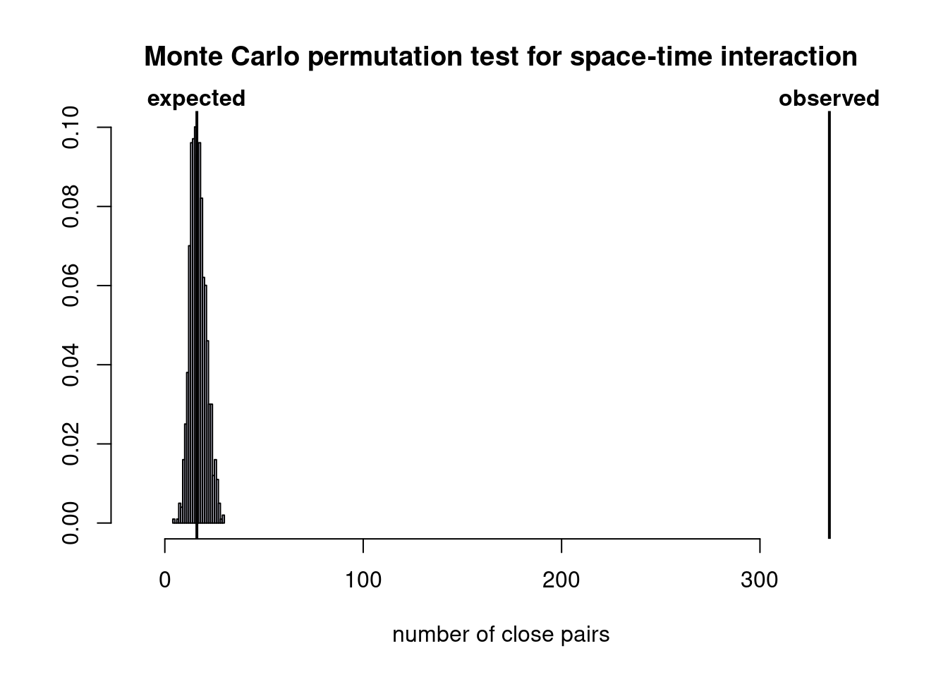
The statistical report suggests that there are 335 pairs of shooting incidents are clustered both spatially and temporally. The observed value leads to p-value of 0.001. This project choose the rule of thumb of p-value threshold to reject null hypothesis of 0.05. Therefore null hypothesis is rejected, there is spatiotemporal aggregation in New York shooting incidents in 2021.
The following two graphs shows the clustered incidents (1) against non clustered incidents (0) and choropleth map of count of clustered incidents by zip code. These two graphs suggests that despite there are many incidents are spatially aggregated, they are not temporally aggregated.
mapView(data_y2d, xcol = "Longitude", ycol = "Latitude", zcol = "CLUSTERED", crs = "+init=epsg:2263") +
mapview(zipcode)mapview(zipcode, zcol = "COUNT")