Introduction

Jakobshavn Isbrae, one of the largest and fastest flowing tidewater glaciers in Greenland, has been exhibiting complex spatiotemporal behaviors. After ~20 years of acceleration, retreating, and thinning, it started to decelerate, readvance, and thicken beginning in 2016. The acceleration and retreat resumed in 2019. Understanding the driving mechanisms of these changes, especially the reversal in 2016, is essential to predict its future contribution to sea-level rise under different scenarios of climate change.

Previous studies found that decreased submarine melt and extended existence of rigid melange as a result of ocean cooling near the terminus are strong candidates for causing the reversal by increasing buttressing at the terminus. Other than forces at the terminus, meltwater runoff at the ice surface can get to the bottom of the glacier through crevasses and moulins, which modulate the ice flow by changing the friction in the interface. This project aims to better understand the relationships of ice surface velocity with meltwater runoff in Jakobshavn Isbrae using linear regression.

Since the industrial revolution, the acceleration of global warming has raised lots of concerns, one of which is the threat from sea-level rise. Greenland tidewater glaciers at the coast are a major contributor to the water input into the ocean. Therefore, a broader scale correlation analysis between the ice velocity of Jakobshavn Isbrae and air temperature over the Greenland ice sheet is conducted here. This study will provide information for identifying the roles of atmospheric circulation in driving the evolution of an important tidewater glacier on the Greenland ice sheet.

Data preparation

Surface ice velocity, runoff, and air temperature at 2m above ice surface in Jakobshavn Isbrae in 2016 are collected from the following sources:

Surface ice velocity maps (GeoTIFFs) with 100m x 100m grids and sporadic temporal resolution from NSIDC: https://nsidc.org/data/nsidc-0481/versions/2
Monthly runoff and air temperature data (netCDF) at 1km x 1km grids are from RACMO2.3p2: https://www.projects.science.uu.nl/iceclimate/models/greenland.php
Drainage basin outline (shapefiles) from NASA: https://earth.gsfc.nasa.gov/cryo/data/polar-altimetry/antarctic-and-greenland-drainage-systems

In this section, the original raster files are cropped to our study area and resampled to a lower resolution for the interest of this study. The code in this section is not evaluated but posted here for reference. Data after the processing in this section can be found in the data directory and will be used in the following analysis.

Load packages

library(tidyverse)
library(reshape2)
library(raster)
library(rasterVis)
library(rgdal)
library(sf)
library(spData)
library(ncdf4)
library(readxl)
library(stats)
library(ggpubr)
library(lubridate)
library(leaflet)
library(httr)
library(jsonlite)

Data preprocessing

## Get and download the velocity Data from NSIDC

# The data has been downloaded to the data directory, to use the api, use your EarthData_taken that can be acquired at https://nsidc.org/support/how/how-request-earthdata-login-token
EarthData_taken = Sys.getenv("EARTHDATA_TOKEN")
url = paste0("https://n5eil02u.ecs.nsidc.org/egi/request?short_name=NSIDC-0481&token=",
             EarthData_taken,
             "&email=yes&version=2&time=2016-01-01T00:00:00,2016-12-31T00:00:00&bounding_box=-52.5,68.8,-47.5,69.5&agent=NO&INCLUDE_META=N&page_size=200&page_num=1")
data = GET(url)

# Download and save data locally
dir.create("data")
file_vel = file(file.path("data", "nsidc0481_16.zip"), "wb") 
writeBin(data$content, file_vel)
close(file_vel)

# Unzip file
data_dir = "data/nsidc0481_16"
dir.create(data_dir)
unzip("data/nsidc0481_16.zip", exdir = data_dir)

## Clean velocity data and crop raster files

data_dir = "data/nsidc0481_16"
names = dir(data_dir, pattern = "^.*vv.*$", full.names = TRUE, recursive = TRUE, ignore.case = TRUE)
names = gsub("^.*68.6.*$", "", names)
names = names[names != ""]
stack_velRaster = stack(names)

# Get dates
date = substr(names, 41, 47)
date = as.Date(format(as.POSIXct(date, format = '%d%b%Y'), "20%y-%m-%d"))
write.csv(date,file="data/vel_Raster_date.csv",row.names=F)

# Crop rasterstack
new_extent = as(extent(-185000, -160000, -2290000, -2272000), 'SpatialPolygons')
crs(new_extent) = crs(stack_velRaster)
stack_velRaster = crop(stack_velRaster, new_extent)

# Save the cropped rasterstack
writeRaster(stack_velRaster, filename="data/stack_velRaster.tif", options="INTERLEAVE=BAND", overwrite=TRUE)

## Preprocess Air temperature data: resample to lower resolution (30 km)

tskin = stack("data/t2m.2016.BN_RACMO2.3p2_ERA5_3h_FGRN055.1km.MM.nc", varname = "t2mcorr")
crs(tskin) = '+proj=stere +lat_0=90 +lat_ts=70 +lon_0=-45 +k=1 +x_0=0 +y_0=0 +datum=WGS84 +units=m +no_defs '
row1 = cbind(-Inf, 150, NA)
row2 = cbind(320, +Inf, NA)
tskin = reclassify(tskin, rbind(row1, row2), right=FALSE)
names(tskin) = month.name

tskin_aggregate <- aggregate(tskin, fact=30)
writeRaster(tskin_aggregate, filename="data/t2m.2016.BN_RACMO2.3p2.tif", options="INTERLEAVE=BAND", overwrite=TRUE)

Data visualization and exploration

Now with raster files having the desired spatial resolution and extent, maps of the monthly averaged velocity, runoff, and air temperature are shown below. All three variables exhibit seasonality and high spatiotemporal variations. Time series of the surface ice velocity is extracted at 6 example locations near the terminus of the glacier.

Surface ice velocity

## Read and visualize the velocity data 

# Read raster data into Rstudio
stack_velRaster = stack("data/stack_velRaster.tif")
date = as.Date(read.csv("data/vel_Raster_date.csv")$x)
stack_velRaster = setZ(stack_velRaster, date)

# Set Z dimension and plot the monthly averaged velocity maps
tmonth = as.numeric(format(getZ(stack_velRaster),"%m"))
stack_velRaster_month = stackApply(stack_velRaster, tmonth, fun = mean)
names(stack_velRaster_month)=month.name
gplot(stack_velRaster_month) + 
  geom_tile(aes(fill = value)) +
  facet_wrap(~variable) +
  scale_fill_distiller(palette = "Spectral") +
  coord_equal() +
  labs(fill = "Velocity (m/year)") +
  theme(axis.text.x = element_text(angle = 45, vjust = 0.5))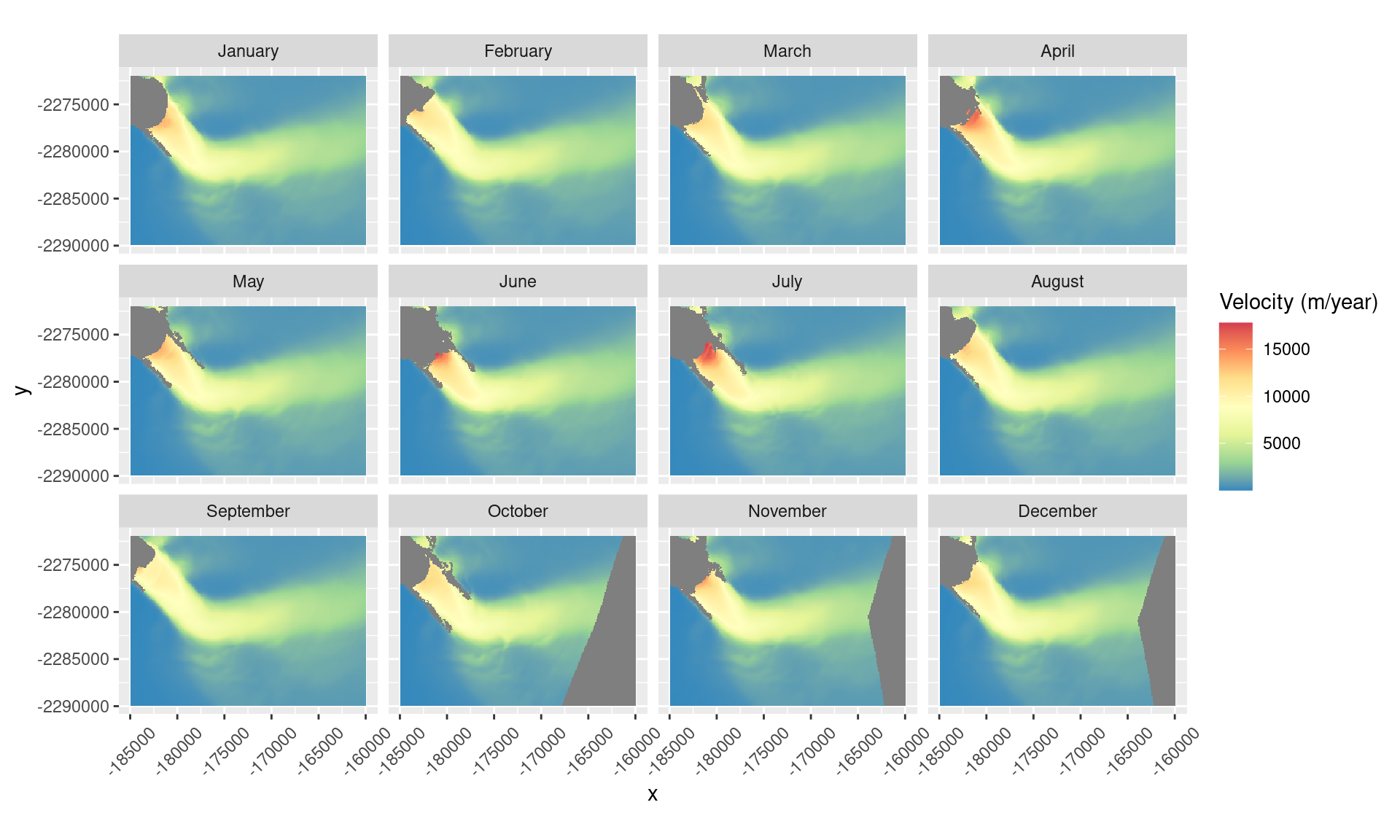

Monthly mean surface ice velocity in 2016

## Extract time series of velocity at the 6 example locations

pts_coord = read_excel("data/Selected_pts.xlsx")
pts = SpatialPoints(data.frame(x=pts_coord$X,y=pts_coord$Y))
projection(pts) = crs(stack_velRaster)

vel = raster::extract(stack_velRaster, pts, buffer=100, fun=mean, na.rm=T)
veldf = as.data.frame(t(vel))
veldf$Date = date
rownames(veldf) <- NULL
veldf = veldf %>%
  arrange(date)

## Interactive map showing the study area

exam_vel = stack_velRaster[[1]]
exmp_pts = spTransform(pts, "+proj=longlat +datum=WGS84 +no_defs")
bed = raster("data/bed_Jakobshavn_egm08.tif")
leaflet() %>% 
  addTiles(group = "OSM") %>%
  addProviderTiles("Esri.WorldImagery", group = "Esri World Imagery") %>%
  addRasterImage(exam_vel, group = "Example velocity map") %>%
  addRasterImage(bed, group = "Bedrock topography") %>%
  addCircleMarkers(data = exmp_pts, label = seq(1,6),
    labelOptions = labelOptions(noHide = TRUE, textsize = "13px", offset=c(0,-10), textOnly = TRUE), group = "Selected points") %>%
  setView(lng = -49.5, lat = 69.1, zoom = 10) %>%
  addLayersControl(baseGroups = c("Esri World Imagery", "OSM"), 
                   overlayGroups = c("Bedrock topography", "Example velocity map", "Selected points"))

Study area with example January velocity map and locations of the velocity time series

## Plot the time series of the surface ice velocity

veldf_plot <- melt(veldf ,  id.vars = 'Date', variable.name = 'series')

# Plot
ggplot(veldf_plot) +
  geom_point(aes(Date, value)) + 
  facet_wrap(series ~ .) +
  theme_bw() +
  labs(y = "Surface ice velocity at point 1 (m/year)") +
  theme(axis.text.x = element_text(angle = 45, vjust = 0.5))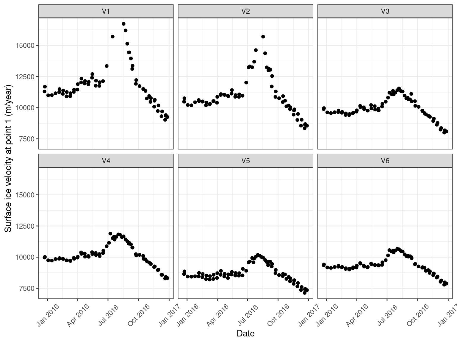

Time series of the surface ice velocity at the 6 example locations

Meltwater runoff

## Read runoff data and resample to the index of velocity time series

runoff = read_excel("data/runoff_sum_abl.xlsx")
runoff_16 = runoff[year(runoff$Date) == 2016,] %>%
  mutate(Date = as.Date(Date))

# Resampling
runoff_interp = as.data.frame(approx(runoff_16$Date,runoff_16$runoff_sum_abl, xout = veldf$Date, 
       rule = 1, method = "linear", ties = mean)) %>%
  rename(Date = "x", runoff = "y")

# Merge with velocity dataframe and only keep the melting season
vel_runoff = left_join(veldf, runoff_interp, by="Date")
## Uncomment the line below to keep the melt season observations only
# vel_runoff = vel_runoff[vel_runoff$runoff > 1000,]
vel_runoff <- subset (vel_runoff, select = -Date)
vel_runoff <- melt(vel_runoff ,  id.vars = 'runoff', variable.name = 'series')

# Plot
ggplot(vel_runoff, aes(x = runoff, y = value)) +
  geom_point() +
  geom_smooth(method='lm') +
  facet_wrap(series ~ ., scales = "free") +
  stat_cor(method = "pearson", label.x.npc = "left", label.y.npc = "top") +
  theme_bw() +
  labs(x = "Runoff (mm.w.e./month)", y = "Surface ice velocity (m/year)")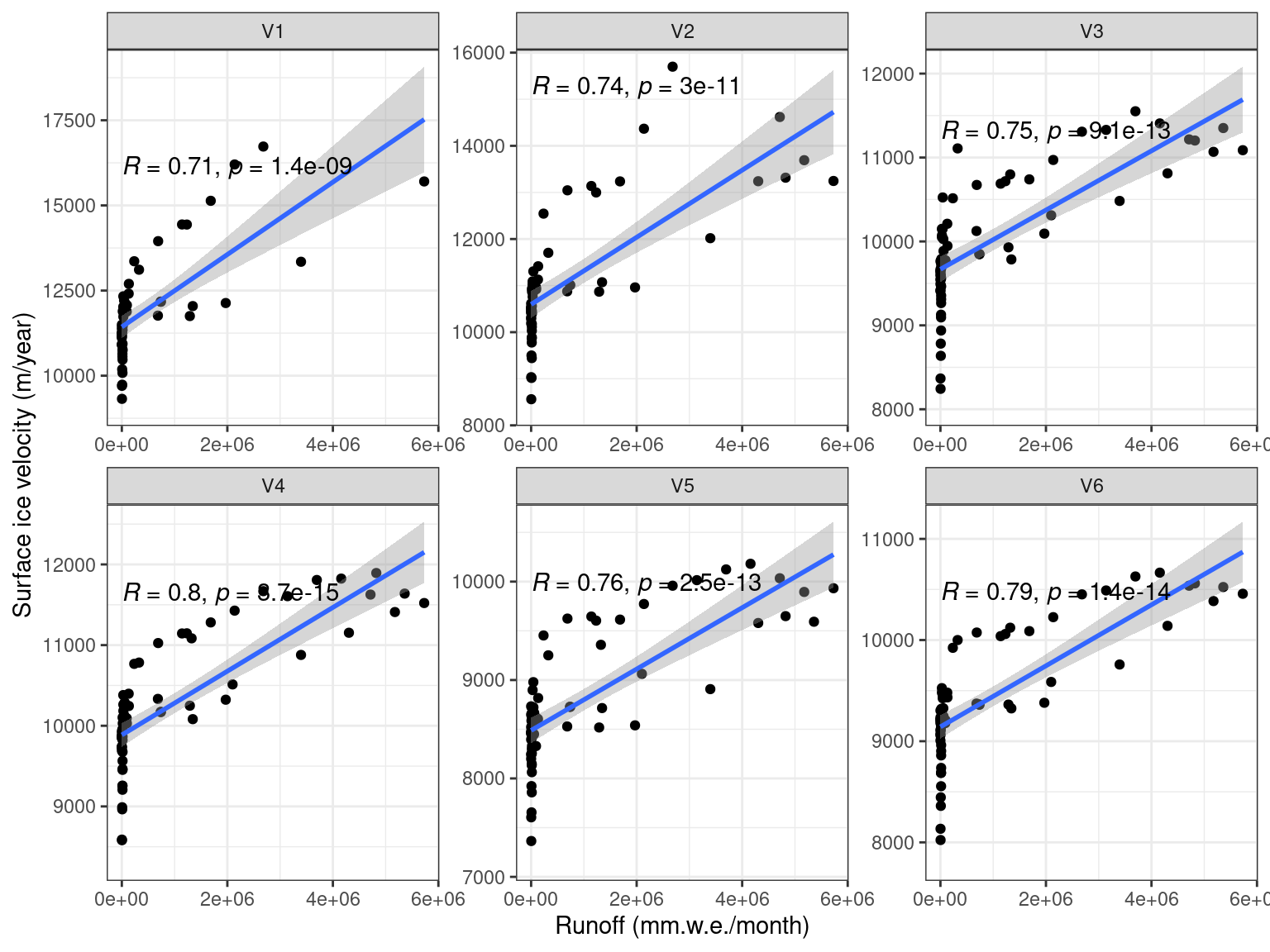

Comparison of time series of surface ice velocity and total runoff in the ablation zone

## Runoff in the study area
runoff = stack("data/runoff_Jakobshavn_2016.nc")
date_r = seq(as.Date("2016-01-01"),length=12,by="months")+14
runoff = setZ(runoff, date_r)
runoff_cropped = crop(runoff, extent(stack_velRaster))

# Resample the rasters to the same spatial resolution (500m x 500m)
velRaster = aggregate(stack_velRaster, fact=5)
runoffRaster = disaggregate(runoff_cropped, fact=2)
names(runoffRaster)=month.name

# Plot
gplot(runoffRaster) + 
  geom_tile(aes(fill = value)) +
  facet_wrap(~variable) +
  scale_fill_distiller(palette = "Spectral") +
  coord_equal() +
  labs(fill = "Runoff (mm.w.e./month)") +
  theme(axis.text.x = element_text(angle = 45, vjust = 0.5))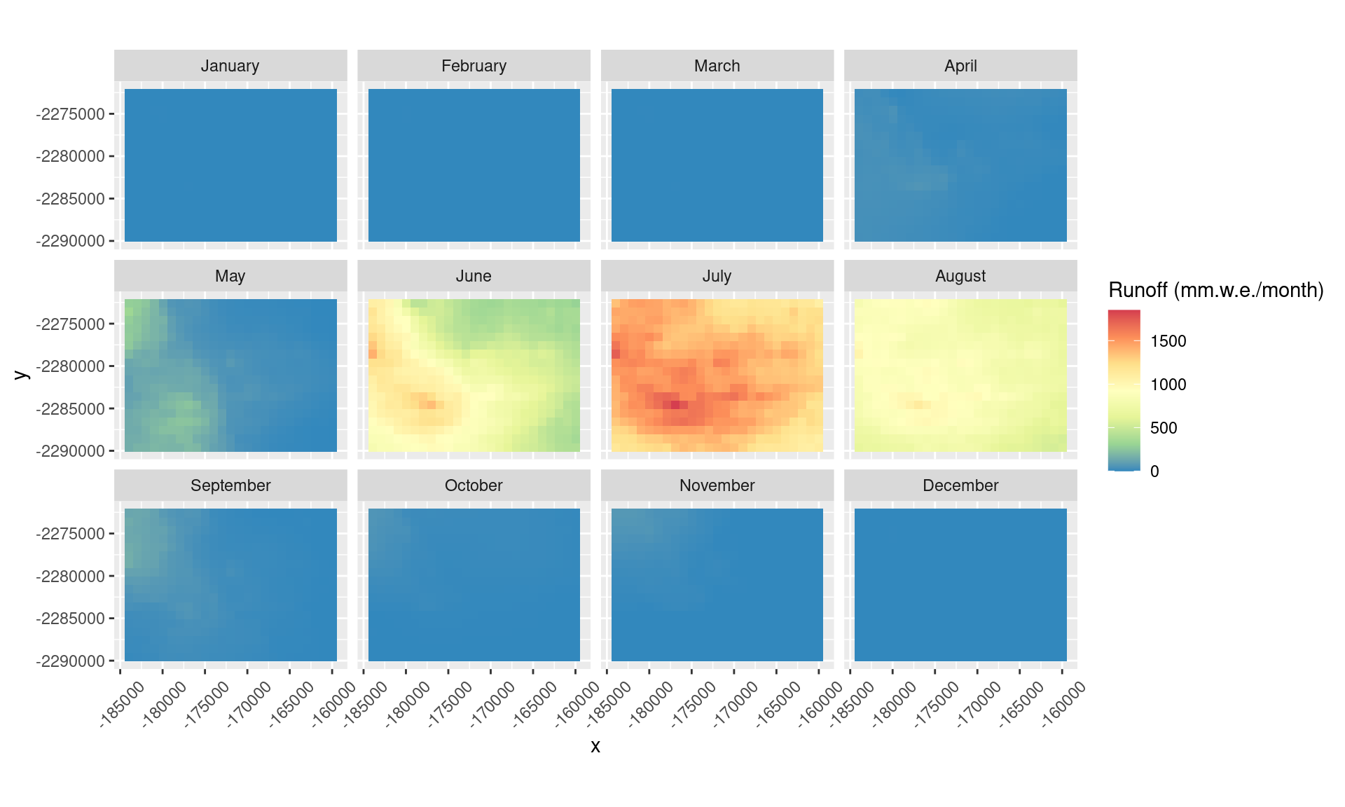

Monthly mean meltwater runoff in 2016

2m air temperature

## 2m air temperature on Greenland

tskin = stack("data/t2m.2016.BN_RACMO2.3p2.tif")
names(tskin) = month.name
offs(tskin)=-273.15

# Plot
gplot(tskin) + 
  geom_tile(aes(fill = value)) +
  facet_wrap(~variable) +
  scale_fill_distiller(palette = "Spectral") +
  coord_equal() +
  labs(fill = "Air temperature (deg C)") +
  theme(axis.text.x = element_text(angle = 45, vjust = 0.5))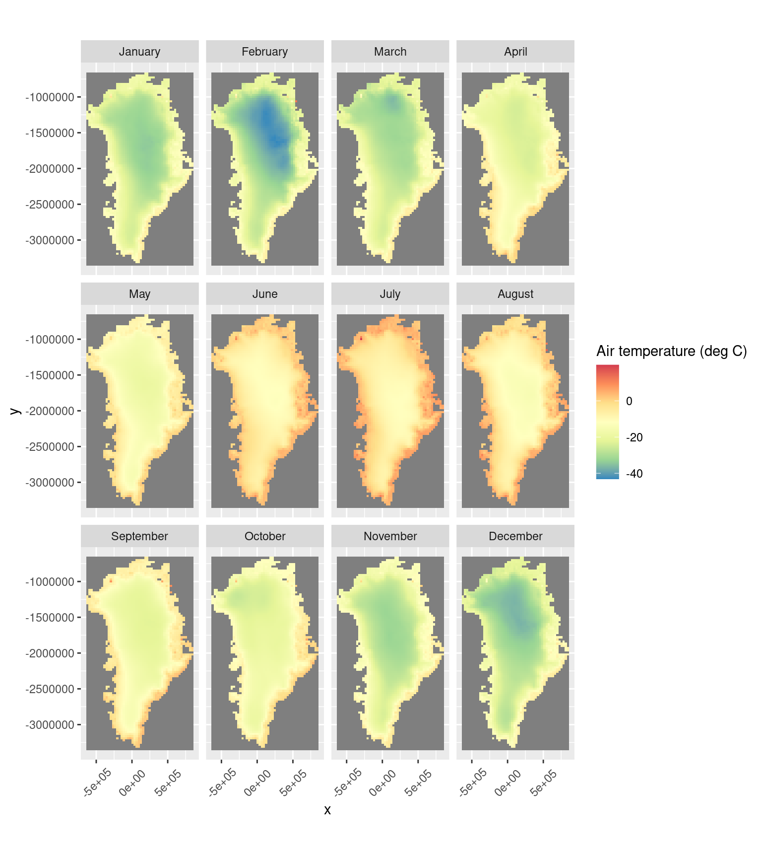

Monthly mean air temperature at 2m above ice surface in 2016

Correlation analysis

In this study, I assume that runoff gets drained to the bed at the place of production and steady-state upstream subglacial drainage. Time series of surface ice velocity and meltwater runoff is extracted at each pixel in 2016 and Pearson correlation coefficients between each pair of time series are calculated. The correlation between surface ice velocity and meltwater runoff is greatest near the terminus and gradually decreases as moving inland along the flow direction. It is likely the lack of seasonality in ice velocity that is responsible for the decreased correlation. The second finding is that the correlation seems to break up in the shear margin especially near the terminus, which indicates a different seasonal pattern of surface ice velocity there. Overall, there is a good correlation between surface ice velocity and meltwater runoff in our study area, especially in the fast-flowing areas. For the areas with low correlations, there is also a good possibility that the assumption doesn’t hold in these regions, which means the meltwater runoff doesn’t reach the ice-bed interface locally and flows above the ice or refreezes in moulins or crevasses.

Correlations between the air temperature at 2 m above ice surface on the Greenland Ice Sheet and surface ice velocity time series at point 1 are shown in the figure below. The correlations are highest on the western and southeastern coast, and also high in southern Greenland. Areas showing good correlations likely have clear seasonal patterns in the air temperature. The spatial correlations patterns provide information for the driving atmospheric forcing of air temperature and glacier mass balance. Future work of comparison with North Atlantic Oscillation (NAO) and Greenland Blocking Index (GBI) is required to continue studying the links between individual tidewater glaciers and the climatic variations.

## Create correlation maps of surface ice velocity and runoff

# Unfold the rasters of velocity and runoff to extract time series at every location
nvel = nlayers(velRaster)
ts_vel = matrix(data=NA, nrow=ncell(velRaster), ncol=nvel)
for(i in 1:nvel){
  ts_vel[,i] = c(as.matrix(velRaster[[i]]))
}
ts_vel = as.data.frame(t(ts_vel))

nrunoff = nlayers(runoffRaster)
ts_runoff = matrix(data=NA, nrow=ncell(runoffRaster), ncol=nrunoff)
for(i in 1:nrunoff){
  ts_runoff[,i] = c(as.matrix(runoffRaster[[i]]))
}
ts_runoff = as.data.frame(t(ts_runoff))

# Resample the runoff time series to the index of velocity time series
# Calculate the Pearson correlation coefficient between the pairs of time series 
ts_runoff_res = matrix(data=NA, nrow=nrow(ts_vel), ncol=ncell(velRaster))
ts_corr = vector()
for(j in 1:ncell(velRaster)){
  if ((sum(ts_runoff[,j]<10) < 8) & (sum(is.na(ts_vel[,j])) < 10)){
    y = approx(date_r,ts_runoff[,j], xout = date, 
               rule = 1, method = "linear", ties = mean)$y
    ts_runoff_res[,j] = y
    ts_corr[j] = cor(y, ts_vel[,j], use = "complete.obs")
  }
  else{
    ts_corr[j] = NA
  }
}
ts_runoff_res = as.data.frame(ts_runoff_res)

# Convert the correlation vector to a raster file
ma_corr = matrix(ts_corr, nrow = nrow(velRaster), ncol = ncol(velRaster))
corr_raster = raster(nrows=nrow(velRaster), ncols=ncol(velRaster))
crs(corr_raster) <- crs(velRaster)
extent(corr_raster) <- extent(velRaster)
values(corr_raster) = ma_corr

# Plot
gplot(corr_raster) +
  geom_tile(aes(fill = value)) +
  labs(fill = "Pearson correlation coefficient") +
  scale_fill_distiller(palette = "Spectral") +
  coord_equal() +
  theme(axis.text.x = element_text(angle = 45, vjust = 0.5))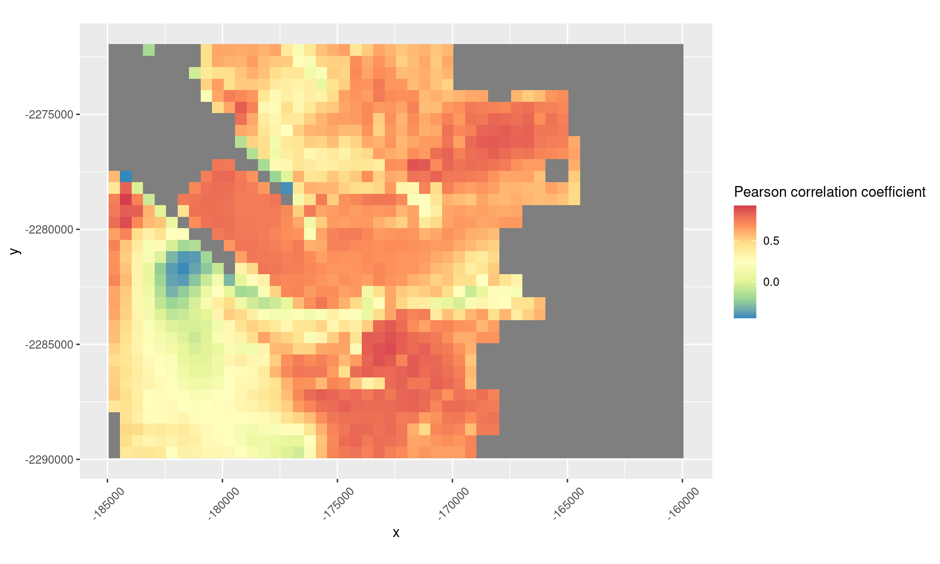

Correlation map of surface ice velocity and runoff in every pixel

## Create correlation maps of surface ice velocity at point 1 with 2m air temperature

# Convert to time series of air temperature at every location
ts_tskin = matrix(data=NA, nrow=ncell(tskin), ncol=12)
for(i in 1:12){
  ts_tskin[,i] = c(as.matrix(tskin[[i]]))
}

ts_tskin = as.data.frame(t(ts_tskin))
ts_tskin$Date = runoff_16$Date

# Resample the air temperature time series to the index of velocity time series
# Calculate the Pearson correlation coefficient between the pairs of time series 
ts_tskin_res = matrix(data=NA, nrow=nrow(veldf), ncol=ncell(tskin))
ts_corr = vector()
for(j in 1:ncell(tskin)){
  if (!all(is.na(ts_tskin[,j]))){
     y = approx(ts_tskin$Date,ts_tskin[,j], xout = veldf$Date, 
                rule = 1, method = "linear", ties = mean)$y
    ts_tskin_res[,j] = y
    ts_corr[j] = cor(y, veldf$V1, use = "complete.obs")
  }
  else{
    ts_corr[j] = NA
  }
}

# Convert the correlation vector to a raster file
ma_corr = matrix(ts_corr, nrow = nrow(tskin), ncol = ncol(tskin))
corr_raster = raster(nrows=nrow(tskin), ncols=ncol(tskin))
crs(corr_raster) <- crs(tskin)
extent(corr_raster) <- extent(tskin)
values(corr_raster) = ma_corr

# Plot
gplot(corr_raster) +
  geom_tile(aes(fill = value)) +
  labs(fill = "Pearson correlation coefficient") +
  scale_fill_distiller(palette = "Spectral") +
  geom_point(data = pts_coord, aes(x = X, y = Y), color = 'black') +
  coord_equal() +
  theme(axis.text.x = element_text(angle = 45, vjust = 0.5))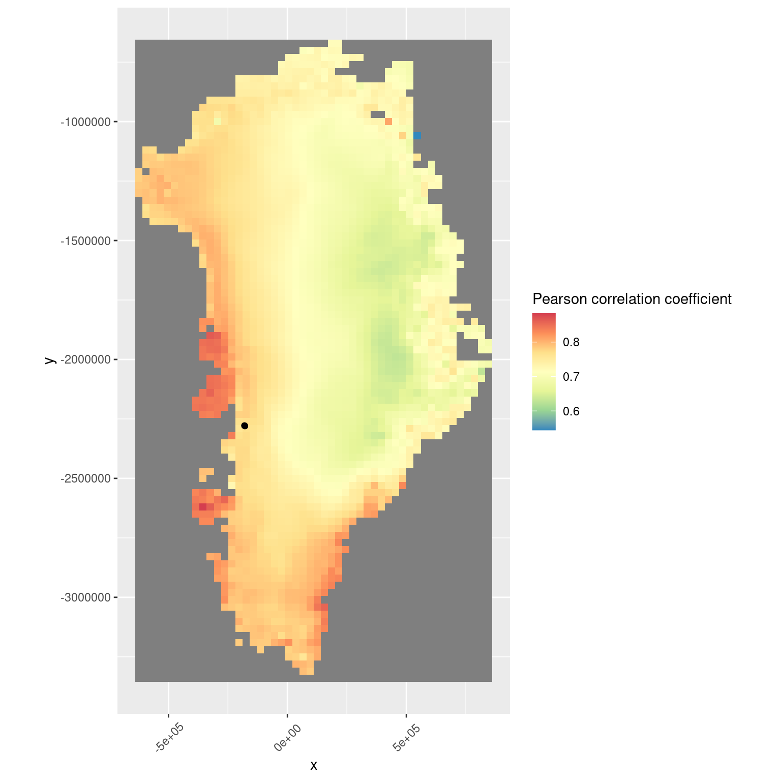

Correlation map of surface ice velocity at point 1 with air temperature

Conclusions

Using correlation analysis on time series of surface ice velocity, meltwater runoff, and air temperature, this study gives a preliminary trial on combining spatial and temporal analysis of the effect of atmospheric forcing on driving the evolution of Jakobshavn Isbrae. Meltwater runoff is highly correlated with surface ice velocity, especially in the fast-flowing region. The correlation decreases in the slow-moving region and shear margin for a number of possible reasons. When comparing the surface ice velocity with air temperature, there is a good correlation (>0.7) in western and southern Greenland, particularly on the coast. Further studies are needed to understand the physical meaning of this result.

For future work, using daily meltwater runoff datasets would be helpful to understand its role in driving the ice flow. Statistically, non-linear correlation and cross-correlation analysis and causal relationship analysis, as well as statistical tests, are needed to reach a firm conclusion. Last but not the least, a better understanding of the runoff distribution and its routing above and below the ice can facilitate the studies with a similar objective as this study.

References

Joughin, I., Smith, B. E., Howat, I. M., Scambos, T., & Moon, T. (2010). Greenland flow variability from ice-sheet-wide velocity mapping. Journal of Glaciology, 56(197), 415–430. https://doi.org/10.3189/002214310792447734
Morlighem, M., Williams, C. N., Rignot, E., An, L., Arndt, J. E., Bamber, J. L., et al. (2017). BedMachine v3: Complete Bed Topography and Ocean Bathymetry Mapping of Greenland From Multibeam Echo Sounding Combined With Mass Conservation. Geophysical Research Letters, 44(21), 11051–11061. https://doi.org/10.1002/2017GL074954
Noel, B., van de Berg, W. J., Lhermitte, S., & van den Broeke, M. R. (2019). Rapid ablation zone expansion amplifies north Greenland mass loss. Science Advances, 5(9), eaaw0123. https://doi.org/10.1126/sciadv.aaw0123
Zwally, H. Jay, Mario B. Giovinetto, Matthew A. Beckley, and Jack L. Saba, 2012, Antarctic and Greenland Drainage Systems, GSFC Cryospheric Sciences Laboratory, at http://icesat4.gsfc.nasa.gov/cryo_data/ant_grn_drainage_systems.php.

Correlation of atmospheric forcing and velocity of Jakobshavn Isbrae

Hui Gao