Tree Population and Median Income in NYC
Mia Giannini
Introduction
This project aims to identify a sort of correlation between median income and tree population among the boroughs of New York City. Lower income communities tend to be more vulnerable to environmental degradation. New York City is one of the big cities facing the urban heat island effect, which is when a metropolitan area experiences a higher climate than surrounding areas due to the excessive population and usage of transportation vehicles. Tree cover is positively correlated with cleaner air, public health, and a more regulated climate. Communities with higher tree coverage are more immune to the effects of climate change, leaving lower income communities to face the full effects. I will be looking at the relationship between the median income of the counties that represent the boroughs of New York and the 2015 NYC Street Tree Census, which gives me the number of street trees per borough.
Materials and methods
The data for this project is sourced from NYC Open Data. It specifically uses the data set entitled ‘2015 Street Tree Census - Tree Data’. This data set was collected by a combination of volunteers and Parks and Recreation staff members resulting in a list of over 680,000 trees as well as over 40 variables pertaining to each tree’s location, health, and overall status. The other data for this project is pulled from the American Community Survey from 2015 using the tidycensus package. I used the tidycensus package to acquire the median income data from 2015 for the counties relative to each borough. I used ggplot to plot the tree population in each borough colored by the median income. I also wanted to show the results of this in map form, by plotting each of the living trees from the dataset onto a map of New York City, colored by the median income of the relative borough.
Start by loading packages
library(tidyverse)
library(tidycensus)
library(readr)
library(dplyr)
library(viridis)
library(ggplot2)
library(mapview)
library(sf)
library(spData)
library(ggmap)
library(maps)
library(mapdata)
library(leaflet)
knitr::opts_chunk$set(cache=TRUE) # cache the results for quick compilingCensus API key
census_api_key(Sys.getenv("CENSUS_API_KEY"), install = TRUE, overwrite = TRUE)## [1] "934de123171c2683ec35d962676bb7341d921db5"readRenviron("~/.Renviron")Read in NYC 2015 Street Tree Census and ACS Census Data
variable <- load_variables(2015, "acs5", cache = TRUE)
nymedinc <- get_acs(geography = "county", state = "NY", county = c("Bronx", "Kings", "New York", "Queens", "Richmond"),
variables = c(medianincome = "B06011_001"), year = 2015)
tree_census_file <- "data/2015_Street_Tree_Census_-_Tree_Data.csv"
if (!file.exists (tree_census_file)) {
dir.create('data')
download.file('https://data.cityofnewyork.us/api/views/uvpi-gqnh/rows.csv?accessType=DOWNLOAD',destfile = tree_census_file)
}
tree_census <- read_csv(tree_census_file)Add borough column to nymedinc
nymedinc$"borough" <- c("Bronx", "Brooklyn", "Manhattan", "Queens", "Staten Island")Filter tree_census for living trees, join with nymedinc and rename ‘tree_data’
tree_data <- tree_census %>%
filter(status == "Alive") %>%
left_join(nymedinc, by=c("borough"="borough"))Summarize the number of trees in each borough
borough_count <- tree_data%>%
group_by(borough)%>%
summarise(count=n())Join borough_count to tree_data, rename tree_pop_data
tree_pop_data <- tree_data %>%
left_join(borough_count, by=c("borough" = "borough"))Results
[~200 words]
Looking at the first graph overall, we can see that Manhattan, the borough with the highest median income actually has the lowest tree population. Staten Island similarly has a higher median income and a tree population on the lower end of things. When we look at the graph as a whole, we can see the the Bronx, Brooklyn, and Queens followed the pattern we expected where the lower income borough has a lower population of trees.
Bar Plot of Tree Population and Median Income
tree_plot <- ggplot(tree_pop_data, aes(x = borough , y= count, fill = estimate))+
geom_bar(stat = "identity")+
scale_fill_gradientn(colors = viridis(256, option = "viridis"))+
labs(x = "Borough", y = "Tree Population", fill = "Median Income", title = "Tree Population and Median Income in NYC Boroughs")
tree_plot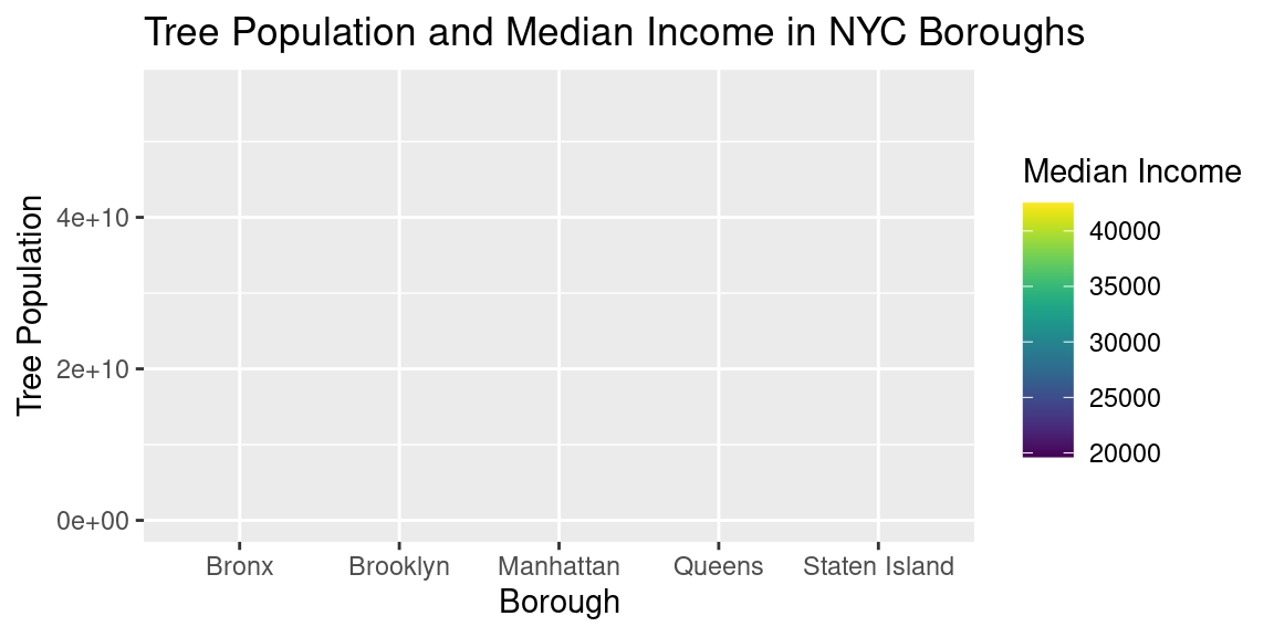
Bar chart of tree population and income data
We see this same data portrayed on the map, allowing us to see and roughly compare the average sizes of each county. We can see that Manhattan has the smallest area compared to the other boroughs, which may have a role in determining the tree population, regardless of median income.
Map of trees, colored by borough
factpal <- colorFactor(topo.colors(5), tree_pop_data$estimate)
map <- leaflet() %>%
addTiles(group = "CartoDB")%>%
addCircleMarkers(data = tree_pop_data, lng = tree_pop_data$longitude, lat = tree_pop_data$latitude, radius = 0.0001, color = ~factpal(estimate))
map