Visualizing the Music of Tom Petty and the Heartbreakers Using R
GEO 511
Sadie Kratt
Introduction
Tom Petty is one of the greatest rock and roll artists of the 20th century. He tragically died in 2017 right after he finished up his final tour. Because Tom Petty is my favorite artist, I have decided to honor him by creating a data visualization of his work through R packages. Music and the information that comes with it is more accessible now than it ever has been. The medium for listening has changed over time from live to recorded, record to tape, and cd to iPod. Streaming services have now taken the lead, allowing users to pay a set amount of money for access to as much or as little music as they’d like at any time. Spotify has emerged as the leading streaming service with 172 million premium users as of mid 2021. Although we have moved away from hard copies, streaming allows artist data to be available and analyzed. Tom Petty and the Heartbreakers may not tour anymore, but their music can continue to present itself through listening, and now visualization.
Questions to be addressed: * How many studio albums did they release and when? * What is the danceability of his songs? * How positive are their songs? * What are the top 10 hits of their career? * Where has the band toured? * What are the top 5 places they have toured?
Materials and Methods
Using the Spotify API, I will be accessing the spotify database to get information about the band. Because Tom Petty produced music both with the band, and as a solo artist, it’s important to note that this is not a comprehensive analysis of his music. This is only a look into the music produced as a band. The artist that is being referred to within the database is “Tom Petty and the Heartbreakers.” Solo work can be found using the artist name “Tom Petty.” All needed artist data will be accessed through this API including the following variables and information: artist name, album name, release date, danceability, valence (positivity), and lyrics.
The Spotifyr package allows you to access and analyze variables included in the API with specific functions. I will be using this package, along with the igraph and ggraph packages to answer the questions listed in the introduction. The graph packages allow users to create graphs from data frames and visualize it in many forms. The graphs that will specifically be shown are dendrograms because they can display a hierarchy of information. The hierarchy will be helpful in showing most often used lyrics per album. I will also be using ggplot2 to show the danceability and positivity of the band’s music.
The spatial component of this analysis will include mapping out the tour locations of the band over the span of their career. This will be used using a crowd sourced list of tour locations and dates found at [The Petty Archives] (https://www.thepettyarchives.com/archives/miscellany/performances/setlists). Using the leaflet package, I will be creating a map of everywhere he’s been, along with a table of dates and how frequent each places was visited. Before creating the maps though, I will be geocoding the areas with the tidygeocoder package and “geocode” function.
Loading the Spotify API
#Load Spotify package and get access
library(spotifyr)
Sys.setenv(SPOTIFY_CLIENT_ID = '097f7729a69e451da9624441ccdb54bd')
Sys.setenv(SPOTIFY_CLIENT_SECRET = 'd1b68552cb2843929b58db9b964f87e9')

access_token <- get_spotify_access_token()
Load Required Packages
library(tidyverse)
library(dplyr)
library(ggplot2)
library(knitr)
library(purrr)
library (tidygeocoder)
library(leaflet)
library(kableExtra)
library(plotly)
knitr::opts_chunk$set(cache=TRUE)  # cache the results for quick compiling
Data Download and Preparation
#load touring data
touring_data <-read.csv('data/locations.csv')
view(touring_data)

#load spotify music data
#Find artist id to access artist information
tom_petty <- get_artist_audio_features("Tom Petty and the Heartbreakers")

#Load album dataset
petty_albums <- get_artist_albums(
  id= "4tX2TplrkIP4v05BNC903e",
  include_groups = c("album", "single", "appears_on", "compilation"),
  market = NULL,
  limit = 20,
  offset = 0,
  authorization = get_spotify_access_token(),
  include_meta_info = FALSE
)
Band Specifics
Number of Albums Released
album_filter <- petty_albums%>%
  filter(name!= c("Mojo Tour Edition", "Hard Promises (Reissue Remastered)",
                  "Damn The Torpedoes (Remastered)",
                   "Damn The Torpedoes (Deluxe Edition)"))%>%
  arrange(desc(release_date))%>%
  select(name, release_date)

kable(album_filter, caption = "Studio Albums")%>%
kable_styling(latex_options = "striped")%>%
scroll_box(width = "600px", height="350px")| name | release_date |
|---|---|
| Angel Dream (Songs and Music From The Motion Picture “She’s The One”) | 2021-06-12 |
| Nobody’s Children | 2015-12-18 |
| Hypnotic Eye | 2014-07-29 |
| Mojo | 2010-06-15 |
| Mojo Tour Edition | 2010-06-15 |
| The Last DJ | 2002-10-08 |
| Echo | 1999-04-13 |
| She’s the One (Songs and Music from the Motion Picture) | 1996-08-06 |
| Into The Great Wide Open | 1991-01-01 |
| Let Me Up (I’ve Had Enough) | 1987-04-21 |
| Pack Up The Plantation: Live! | 1985-11-26 |
| Southern Accents | 1985-03-26 |
| Long After Dark | 1982-11-02 |
| Hard Promises (Reissue Remastered) | 1981-05-05 |
| Hard Promises | 1981-05-05 |
| Damn The Torpedoes | 1979-10-19 |
| Damn The Torpedoes (Remastered) | 1979-10-19 |
| Damn The Torpedoes (Deluxe Edition) | 1979-10-19 |
| You’re Gonna Get it | 1978-05-02 |
number_albums <- count(album_filter)
number_albums
## n
## 1 19The band put out a total of 19 studio albums which includes live and deluxe versions. This does not include solo albums put out by Tom Petty, though they should be considered due to band members playing on those albums and fans associating both band and solo work together.
Danceability
var_width = 20

petty_filter <-tom_petty%>%
  select(album_name, danceability)%>%
  dplyr::mutate(album_wrap=str_wrap(album_name, width = var_width))


album_dance <- ggplot(petty_filter, aes(x=danceability, fill=album_wrap,
                      text = paste(album_name))) +
  geom_density(alpha=0.7, color=NA) +
  ggtitle("Danceability by Album") +
  labs(x="Danceability", y="Density") +
  guides(fill=guide_legend(title="Album Name")) +
  theme_minimal() +
    theme(legend.position="none",
          strip.text.x = element_text(size = 8)) +
    facet_wrap(~ album_wrap)
album_dance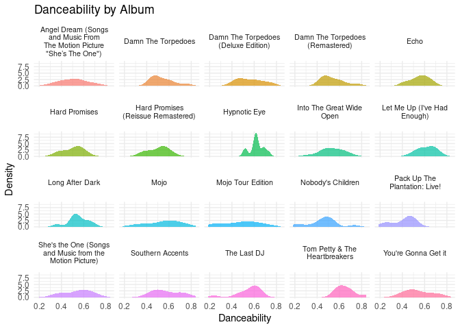
“Danceability describes how suitable a track is for dancing based on a combination of musical elements including tempo, rhythm stability, beat strength, and overall regularity. A value of 0.0 is least danceable and 1.0 is most danceable.” (Plantinga, 2018). This one surprised me most because I expected “Damn The Torpedoes” to have the highest danceability. This album was a breakthrough album with many upbeat, well-known songs. But looking at this, it seems like “She’s the One” and “Hypnotic Eye” have the highest throughout their albums. This reinforces the idea that there is more to songs than just being a fun or upbeat sound.
Valence
#Positivity of songs
petty_valence <- tom_petty%>%
  arrange(-valence) %>%
  select(.data$track_name, .data$valence) %>%
  distinct()%>%
  head(10)
petty_valence
## track_name valence
## 1 Rockin' Around (With You) 0.970
## 2 Don't Do Me Like That 0.961
## 3 Anything That's Rock 'n' Roll 0.950
## 4 Learning To Fly 0.949
## 5 Change Of Heart 0.941
## 6 Jammin' Me 0.938
## 7 The Same Old You 0.931
## 8 Don't Come Around Here No More 0.922
## 9 Accused of Love 0.911
## 10 We Stand A Chance 0.903valence_plot <- ggplot(petty_valence, aes(x = reorder(track_name, -valence),
valence, text = paste(valence))) +
geom_point(color="#7625be") +
theme(axis.text.x = element_text(color="grey30",
size=8, angle=40),
axis.text.y = element_text(face="bold", color="grey30",
size=10,),
axis.title = element_text(color = "#7625be", face = "bold")) +
ggtitle("Top 10 Positive Songs") +
xlab("Track Name") +
ylab("Valence")
ggplotly(valence_plot, tooltip=c("text"))Valence is “a measure from 0.0 to 1.0 describing the musical positiveness conveyed by a track. Tracks with high valence sound more positive (e.g. happy, cheerful, euphoric), while tracks with low valence sound more negative (e.g. sad, depressed, angry).” (Plantinga, 2018) These results are not surprising because they all are upbeat tempos with generally happy lyrics.
Top 10 Hits
top_ten <- get_artist_top_tracks(
  id= "4tX2TplrkIP4v05BNC903e",
  market = "US",
  authorization = get_spotify_access_token(),
  include_meta_info = FALSE
)%>%
  select(name, album.name)
colnames(top_ten) = c("Song", "Album")
top_ten
## Song Album
## 1 American Girl Tom Petty & The Heartbreakers
## 2 Mary Jane's Last Dance Greatest Hits
## 3 Learning To Fly Into The Great Wide Open
## 4 Refugee Damn The Torpedoes (Deluxe Edition)
## 5 Breakdown Tom Petty & The Heartbreakers
## 6 Christmas All Over Again A Very Special Christmas 2
## 7 Don't Do Me Like That Damn The Torpedoes (Deluxe Edition)
## 8 Into The Great Wide Open Into The Great Wide Open
## 9 Don't Come Around Here No More Southern Accents
## 10 Here Comes My Girl Damn The Torpedoes (Deluxe Edition)kable(top_ten, caption = "Top 10 Tracks") %>%
row_spec(c(1,3,5,7,9),background = "#Cab5dc")%>%
kable_styling(latex_options = "striped")| Song | Album |
|---|---|
| American Girl | Tom Petty & The Heartbreakers |
| Mary Jane’s Last Dance | Greatest Hits |
| Learning To Fly | Into The Great Wide Open |
| Refugee | Damn The Torpedoes (Deluxe Edition) |
| Breakdown | Tom Petty & The Heartbreakers |
| Christmas All Over Again | A Very Special Christmas 2 |
| Don’t Do Me Like That | Damn The Torpedoes (Deluxe Edition) |
| Into The Great Wide Open | Into The Great Wide Open |
| Don’t Come Around Here No More | Southern Accents |
| Here Comes My Girl | Damn The Torpedoes (Deluxe Edition) |
The top 10 tracks to be found are what was expected. All songs except for “Christmas All Over Again” appear on the Greatest Hits album and were released as singles for their respective albums.
Where Did They Tour?
Geocode locations
touring_geo <- touring_data %>% geocode (City, method = 'osm', lat = latitude , long = longitude)%>%
write_csv(file="data/touring_geo.csv")touring_geo=read_csv("data/touring_geo.csv")## Rows: 1434 Columns: 7## ── Column specification ────────────────────────────────────────────────────────
## Delimiter: ","
## chr (5): ï..Date, Venue, City, Extras, Notes
## dbl (2): latitude, longitude##
## ℹ Use `spec()` to retrieve the full column specification for this data.
## ℹ Specify the column types or set `show_col_types = FALSE` to quiet this message.Mapping Locations with Leaflet
map_tour <- leaflet(touring_geo) %>%
  addProviderTiles("CartoDB.Positron") %>%
  addCircleMarkers(radius = 1, popup = touring_geo$City,
                   color = "#7625be", clusterOptions = markerClusterOptions())
## Assuming "longitude" and "latitude" are longitude and latitude, respectively## Warning in validateCoords(lng, lat, funcName): Data contains 161 rows with
## either missing or invalid lat/lon values and will be ignoredmap_tourWhere are the top 5 locations visited while touring?
top_5<-touring_geo%>%
  filter(City != "NA")%>%
  count(City)%>%
  arrange(desc(n))
top_5
## # A tibble: 382 × 2
## City n
## <chr> <int>
## 1 New York City, New York 42
## 2 San Francisco, California 41
## 3 Philadelphia, Pennsylvania 23
## 4 West Hollywood, California 23
## 5 London, England 22
## 6 Los Angeles, California 22
## 7 Atlanta, Georgia 21
## 8 Chicago, Illinois 21
## 9 Dallas, Texas 18
## 10 Milwaukee, Wisconsin 17
## # … with 372 more rowskable(top_5, caption = "Top 5 Touring Locations") %>%
kable_styling(latex_options = "striped")%>%
row_spec(1:5, background = "#Cab5dc")%>%
scroll_box(width = "600px", height="350px")| City | n |
|---|---|
| New York City, New York | 42 |
| San Francisco, California | 41 |
| Philadelphia, Pennsylvania | 23 |
| West Hollywood, California | 23 |
| London, England | 22 |
| Los Angeles, California | 22 |
| Atlanta, Georgia | 21 |
| Chicago, Illinois | 21 |
| Dallas, Texas | 18 |
| Milwaukee, Wisconsin | 17 |
| Austin, Texas | 16 |
| Universal City, California | 15 |
| Morrison, Colorado | 14 |
| San Diego, California | 14 |
| Tampa, Florida | 14 |
| Berkeley, California | 13 |
| Clarkson, Michigan | 13 |
| Phoenix, Arizona | 13 |
| Pittsburgh, Pennsylvania | 13 |
| Sacramento, California | 13 |
| Mountain View, California | 12 |
| Saratoga Springs, New York | 12 |
| Indianapolis, Indiana | 11 |
| Kansas City, Missouri | 11 |
| Portland, Oregon | 11 |
| Seattle, Washington | 11 |
| Cincinnati, Ohio | 10 |
| Denver, Colorado | 10 |
| Hartford, Connecticut | 10 |
| Holmdel, New Jersey | 10 |
| Houston, Texas | 10 |
| Toronto, Ontario | 10 |
| Columbus, Ohio | 9 |
| Cuyahoga Falls, Ohio | 9 |
| George, Washington | 9 |
| Hollywood, California | 9 |
| Raleigh, North Carolina | 9 |
| St. Louis, Missouri | 9 |
| Boston, Massachusetts | 8 |
| Charlotte, North Carolina | 8 |
| Cleveland, Ohio | 8 |
| Columbia, Maryland | 8 |
| Irvine, California | 8 |
| Las Vegas, Nevada | 8 |
| Memphis, Tennessee | 8 |
| Nashville, Tennessee | 8 |
| Noblesville, Indiana | 8 |
| Reno, Nevada | 8 |
| Santa Cruz, California | 8 |
| Sydney, Australia | 8 |
| Wantagh, New York | 8 |
| Birmingham, England | 7 |
| Costa Mesa, California | 7 |
| Detroit, Michigan | 7 |
| Minneapolis, Minnesota | 7 |
| Omaha, Nebraska | 7 |
| St. Paul, Minnesota | 7 |
| The Woodlands, Texas | 7 |
| Vancouver, British Columbia | 7 |
| West Palm Beach, Florida | 7 |
| Auburn Hills, Michigan | 6 |
| Darien Lake, New York | 6 |
| East Rutherford, New Jersey | 6 |
| Gainesville, Florida | 6 |
| Hoffman Estates, Illinois | 6 |
| Maryland Heights, Missouri | 6 |
| Oakland, California | 6 |
| Uniondale, New York | 6 |
| Boston, Massachussetts | 5 |
| Bristow, Virginia | 5 |
| Louisville, Kentucky | 5 |
| Mansfield, Massachusetts | 5 |
| Mansfield, Massachussetts | 5 |
| Melbourne, Australia | 5 |
| Miami, Florida | 5 |
| Oklahoma City, Oklahoma | 5 |
| Orlando, Florida | 5 |
| Paris, France | 5 |
| Santa Barbara, California | 5 |
| Santa Monica, California | 5 |
| St. Petersburg, Florida | 5 |
| Tokyo, Japan | 5 |
| Tuscon, Arizona | 5 |
| Albany, New York | 4 |
| Bloomington, Minnesota | 4 |
| Bonner Springs, Kansas | 4 |
| Brussels, Belgium | 4 |
| Burgettstown, Pennsylvania | 4 |
| Camden, New Jersey | 4 |
| Concord, California | 4 |
| Devore, California | 4 |
| East Troy, Wisconsin | 4 |
| Grand Rapids, Michigan | 4 |
| Hamburg, Germany | 4 |
| Manchester, England | 4 |
| New Haven, Connecticut | 4 |
| New Orleans, Louisiana | 4 |
| Northridge, California | 4 |
| Providence, Rhode Island | 4 |
| Stockholm, Sweden | 4 |
| Tempe, Arizona | 4 |
| Tulsa, Oklahoma | 4 |
| Washington, D.C. | 4 |
| Antioch, Tennessee | 3 |
| Brisbane, Australia | 3 |
| Buffalo, New York | 3 |
| Calgary, Alberta | 3 |
| Darien Center, New York | 3 |
| Dublin, Ireland | 3 |
| Edmonton, Alberta | 3 |
| Inglewood, California | 3 |
| Jacksonville, Florida | 3 |
| Palo Alto, California | 3 |
| Richfield, Ohio | 3 |
| Rochester, New York | 3 |
| Scranton, Pennsylvania | 3 |
| Syracuse, New York | 3 |
| Tinley Park, Illinois | 3 |
| Winnipeg, Manitoba | 3 |
| Adelaide, Australia | 2 |
| Akron, Ohio | 2 |
| Albuquerque, New Mexico | 2 |
| Allentown, Pennsylvania | 2 |
| Alpine, California | 2 |
| Ames, Iowa | 2 |
| Angels Camp, California | 2 |
| Bakersfield, California | 2 |
| Basel, Switzerland | 2 |
| Berlin, Germany | 2 |
| Binghamton, New York | 2 |
| Boise, Idaho | 2 |
| Brighton, England | 2 |
| Carbondale, Illinois | 2 |
| Cardiff, Wales | 2 |
| Cedar Rapids, Iowa | 2 |
| Champaign, Illinois | 2 |
| Chula Vista, California | 2 |
| Cologne, Germany | 2 |
| Daly City, California | 2 |
| Des Moines, Iowa | 2 |
| Edinburgh, Scotland | 2 |
| Estero, Florida | 2 |
| Eugene, Oregon | 2 |
| Evansville, Indiana | 2 |
| Fairfax, Virginia | 2 |
| Forest Hills, New York | 2 |
| Fort Wayne, Indiana | 2 |
| Frankfurt, Germany | 2 |
| Fresno, California | 2 |
| Glasgow, Scotland | 2 |
| Hershey, Pennsylvania | 2 |
| Lexington, Kentucky | 2 |
| Madison, Wisconsin | 2 |
| Malibu, California | 2 |
| Manchester, New Hampshire | 2 |
| Manchester, Tennessee | 2 |
| Mannheim, Germany | 2 |
| Mansfield, Massachussets | 2 |
| Maple, Ontario | 2 |
| Moline, Illinois | 2 |
| Montreal, Quebec | 2 |
| Munich, Germany | 2 |
| Nagoya, Japan | 2 |
| New Orleans, Lousiana | 2 |
| Newark, New Jersey | 2 |
| Noblesville, Illinois | 2 |
| Norman, Oklahoma | 2 |
| Osaka, Japan | 2 |
| Oslo, Norway | 2 |
| Ottawa, Ontario | 2 |
| Pasadena, California | 2 |
| Paso Robles, California | 2 |
| Pelham, Alabama | 2 |
| Peoria, Illinois | 2 |
| Perth, Australia | 2 |
| Philadelphia, Pennsylvania | 2 |
| Portsmouth, Virginia | 2 |
| San Antonio, Texas | 2 |
| Saskatoon, Saskatchewan | 2 |
| St. John’s, Newfoundland | 2 |
| Tacoma, Washington | 2 |
| Vancouver, Canada | 2 |
| Ventura, California | 2 |
| – | 1 |
| –, Belgium | 1 |
| Alpharetta, Georgia | 1 |
| Amsterdam, Netherlands | 1 |
| Amsterdam, The Netherlands | 1 |
| Anaheim, California | 1 |
| Arrington, Virginia | 1 |
| Asbury Park, New Jersey | 1 |
| Aspen, Colorado | 1 |
| Atlantic City, New Jersey | 1 |
| Auckland, New Zealand | 1 |
| Augusta, Maine | 1 |
| Aylesbury, England | 1 |
| Baltimore, Maryland | 1 |
| Baton Rouge, Louisiana | 1 |
| Belfast, Ireland | 1 |
| Bethehem, Pennsylvania | 1 |
| Bethlehem, Pennsylvania | 1 |
| Birmingham, Alabama | 1 |
| Bismarck, North Dakota | 1 |
| Bloomington, Indiana | 1 |
| Boston, Massachussets | 1 |
| Boston, Massachusetts | 1 |
| Boulder, Colorado | 1 |
| Bozeman, Montana | 1 |
| Bristol, Connecticut | 1 |
| Bristol, England | 1 |
| Broomfield, Colorado | 1 |
| Burbank, California | 1 |
| Burgettstown, Pennsylvania | 1 |
| Burggetstown, Pennsylvania | 1 |
| Caddot, Wisconsin | 1 |
| Canandaigua, New York | 1 |
| Chapel Hill, North Carolina | 1 |
| Charleston, South Carolina | 1 |
| Charlevoix, Michigan | 1 |
| Charlotte, Noorth Carolina | 1 |
| Chicago, Ilinois | 1 |
| Chicao, Illinois | 1 |
| Chico, California | 1 |
| Chillicothe, Illinois | 1 |
| Christchurch, New Zealand | 1 |
| Cincinnati, Ohio. Liberty went! | 1 |
| Colorado Springs, Colorado | 1 |
| Columbia, South Carolina | 1 |
| Columbus, Georgia | 1 |
| Copenhagen, Denmark | 1 |
| Cork, Ireland | 1 |
| Corvallis, Oregon | 1 |
| Council Bluffs, Iowa | 1 |
| Coventry, England | 1 |
| Cuyahoga Fals, Ohio | 1 |
| Dana Point, California | 1 |
| Davis, California | 1 |
| Dayton, Ohio | 1 |
| Daytona Beach, Florida | 1 |
| Del Mar, California | 1 |
| Dortmund, Germany | 1 |
| Dortmund, West Germany | 1 |
| Dover, Delaware | 1 |
| Duluth, Minnesota | 1 |
| East Berlin, East Germany | 1 |
| East Hampton, New York | 1 |
| East Rutherford, New Jersey | 1 |
| Easy Troy, Wisconsin | 1 |
| El Paso, Texas | 1 |
| Englewood, Colorado | 1 |
| Essen, Germany | 1 |
| Exeter, england | 1 |
| Fort Myers, Florida | 1 |
| Frankfurt, West Germany | 1 |
| Garden City, Long Island, New York | 1 |
| Geleen, Netherlands | 1 |
| George, Washingon | 1 |
| Glendale, Arizona | 1 |
| Gothenburgh, Sweden | 1 |
| Gothernbeg, Sweden | 1 |
| Greenville, South Carolina | 1 |
| Gulf Shores, Alabama | 1 |
| Halifax, Nova Scotia | 1 |
| Hanover, West Germany | 1 |
| Hartford, Connecticut | 1 |
| Helsinki, Finland | 1 |
| Hempstead, New York | 1 |
| Hertfordshire, England | 1 |
| Honolulu, Hawaii | 1 |
| Horsens, Denmark | 1 |
| Hunter Mountain, New York | 1 |
| Huntsville, Alabama | 1 |
| Indian Wells, California | 1 |
| Iowa City, Iowa | 1 |
| Jackson Hole, Wyoming | 1 |
| Jackson, Mississippi | 1 |
| Jerusalem, Israel | 1 |
| Kansas City, Kansas | 1 |
| Kingston Upon Hull, England | 1 |
| Knoxville, Tennessee | 1 |
| Lakeland, Florida | 1 |
| Lancaster, England | 1 |
| Landover, Maryland | 1 |
| Las Cruches, New Mexico | 1 |
| Leeds, England | 1 |
| Little Rock, Arkansas | 1 |
| Liverpool, England | 1 |
| Locarno, Switzerland | 1 |
| London, Ontario | 1 |
| Los Angeles, California | 1 |
| Lucca, Italy | 1 |
| Lund, Sweden | 1 |
| Malmo, Sweden | 1 |
| Mankato, Minnesota | 1 |
| Mansfield, Massachusetts | 1 |
| Marsyville, California | 1 |
| Middletown, New York | 1 |
| Milano, Italy | 1 |
| Moderna, Italy | 1 |
| Munich, West Germany | 1 |
| Nampa, Idaho | 1 |
| Napa, California | 1 |
| Nashville, Tennesee | 1 |
| Newcastle upon Tyne, England | 1 |
| Newport, England | 1 |
| Nogent-sur-Marne, France | 1 |
| Norfolk, Virginia | 1 |
| Normal, Illinois | 1 |
| North Charleston, South Carolina | 1 |
| North Little Rock, Arkansas | 1 |
| Nuremberg, Germany | 1 |
| Nuremberg, West Germany | 1 |
| Offenbach, Germany | 1 |
| Oklahome City, Oklahoma | 1 |
| Oklahome City, Oklahome | 1 |
| Omaha, Missouri | 1 |
| Oxford, England | 1 |
| Painesville, Ohio | 1 |
| Passaic, New Jersey | 1 |
| Pemberton, British Columbia | 1 |
| Pembroke Pines, Florida | 1 |
| Pensacola, Florida | 1 |
| Philadelphia, Pennslylvania | 1 |
| Philadelphia, Pennsylvania | 1 |
| Port Chester, New York | 1 |
| Portland, Maine | 1 |
| Randall’s Island, New York | 1 |
| Rapid City, South Dakota | 1 |
| Redding, California | 1 |
| Reseda, California | 1 |
| Richmond, Virginia | 1 |
| Richmond. Virginia | 1 |
| Riverside, California | 1 |
| Rome, Italy | 1 |
| Rosemont, Illinois | 1 |
| Roslyn, New York | 1 |
| Rotterdam, The Netherlands | 1 |
| Royal Oak, Michigan | 1 |
| Salinas, California | 1 |
| Salt Lake City, Utah | 1 |
| San Diego, Calfornia | 1 |
| San Jose, California | 1 |
| Santa Ana, California | 1 |
| Santa Rosa, California | 1 |
| Saratofa Springs, New York | 1 |
| Sausalito, California | 1 |
| Savannah, Georgia | 1 |
| Selma, Texas | 1 |
| Sheffield, England | 1 |
| Shreveport, Louisiana | 1 |
| Sioux Falls, South Dakota | 1 |
| South Bard, Indiana | 1 |
| South Yarmouth, Massachussetts | 1 |
| Southampton, New York | 1 |
| Spokane, Washington | 1 |
| Springfield, Missouri | 1 |
| Stoke on Trent, England | 1 |
| Sturgis, South Dakota | 1 |
| Stuttgart, West Germany | 1 |
| Sunrise, Florida | 1 |
| Tel-Aviv, Israel | 1 |
| The Woodslads, Texas | 1 |
| Toledo, Ohio | 1 |
| Tupelo, Mississippi | 1 |
| Turin, Italy | 1 |
| Tuscaloosa, Alabama | 1 |
| Uncasville, Connecticut | 1 |
| Universal City, Los Angeles | 1 |
| Utrecht, Netherlands | 1 |
| Verona, Italy | 1 |
| Virginia Beach, Virginia | 1 |
| Washington, DC | 1 |
| Wellington, New Zealand | 1 |
| Wellington, New Zealand | 1 |
| West Valley City, Utah | 1 |
| Wichita, Kansas | 1 |
| Willamsburg, Virginia | 1 |
| Williamsburg, Virginia | 1 |
| Wolverhampton, England | 1 |
| Worcester, Massachusetts | 1 |
| Worchester, Massachussetts | 1 |
| Yakima, Washington | 1 |
The top touring locations were found to be NYC, San Francisco, Philadelphia, West Hollywood, and London. One of the interesting parts of this information is that the two top cities were visited twice as many times as the next three. This would make sense though due to New York’s large population and many concert venues. As for California, the band became what they were there after relocating from Gainsville, Florida. You can hear this place influence in many of their songs, and now see that they always toured back home.
Conclusions
The Spotify API allows for a better understanding of the artists we love in more ways than just listening. By using R, I was able to gain a new understanding of my favorite artist and learn ways to interpret data. Visualizing the places Tom Petty toured allows fans to see how far his influence reached. Making playlists for new listeners also becomes easier by assessing what kind of listener they are. If they like hits that make you happy, I would recommend them to listen to “Don’t do me Like That.” One of the drawbacks of this project though is the singularity of artists. Tom Petty, and many other artists, put out music under a solo label in addition to their band. Unless you merge the data frames, you only get a view of part of their work. In order to get a full look at Tom’s music, you would have to merge his solo work, band work, and “Mudcrutch” work. Overall though, this API is very useful and very unique to work with.
References
Aimee, W. (n.d.). Tour Dates and Setlists - The Petty Archives. Retrieved December 9, 2021, from www.thepettyarchives.com website: https://www.thepettyarchives.com/archives/miscellany/performances/setlists charlie86. (2021, December 2). spotifyr. Retrieved December 9, 2021, from GitHub website: https://github.com/charlie86/spotifyr DataCamp. (n.d.). spotifyr package - RDocumentation. Retrieved December 9, 2021, from www.rdocumentation.org website: https://www.rdocumentation.org/packages/spotifyr/versions/2.2.1 Holtz, Y. (2018). Dendrogram customization with R and ggraph. Retrieved December 9, 2021, from www.r-graph-gallery.com website: https://www.r-graph-gallery.com/335-custom-ggraph-dendrogram.html Pedersen, T. L. (2021, December 2). ggraph. Retrieved December 9, 2021, from GitHub website: https://github.com/thomasp85/ggraph Plantinga, B. (2018, April 29). What do Spotify’s audio features tell us about this year’s Eurovision Song Contest? Retrieved from Medium website: https://medium.com/@boplantinga/what-do-spotifys-audio-features-tell-us-about-this-year-s-eurovision-song-contest-66ad188e112a *Statista. (2018). Spotify users - subscribers in 2018 | Statista. Retrieved from Statista website: https://www.statista.com/statistics/244995/number-of-paying-spotify-subscribers/