Stay safe!
Visualizing the Crime Incidents in Buffalo, NY (2010-2020)
Exploring the spatiotemporal pattern of crime incidents and the correlation with sociodemographic characteristics in the City of Buffalo, New York
Wei Liu
1 Introduction
Crime, as what it always appears to be, is the negative power in our society that tends to trigger multiple problems. With the increasing demand for higher quality of life in the modern world, the general public attaches more attention to the safety of the living environment as one of the basic factors considered. There has been considerable effort extended to exploring and understanding the pattern of various types of crimes. There exists a sub-field, namely, geographic profiling, which is the marginal subject of criminology and geography, looking into the crime events with both the theoretical basics from criminology and spatial methodologies from geography, with the ultimate goal of promoting suggestions for reducing crime rates and maintaining social safety.
In this project, we want to reveal and understand the spatiotemporal distribution of crime incidents in Buffalo, New York. We are going to achieve our objective mainly by visualization of the crime incidents over time as well as over the study region. Besides, we also want to detect the relationship between crime and corresponding sociodemographic attributes in each defined area. The contribution of this project can be three-folded:
Firstly, we analyze the pattern of crime incidents in Buffalo, NY from multiple dimensions through innovative approaches.
Secondly, we further explore the potential mechanism behind the scene which may play a role in the formation of crime incidents.
Thirdly, based on the aforementioned results, we are able to provide useful suggestions for promoting overall social safety.
2 Data and methods
2.1 Data
1. Crime incidents
The csv file of crime incidents is in the public domain, available from the website of Open Data Portal of the City of Buffalo.
2. Census Block Groups (CBGs) 2010 of the City of Buffalo
The Census Block Groups 2010 data is available from Buffalo Open Data Portal. CBGs are statistical divisions of census tracts, are generally defined to contain between 600 and 3,000 people, and are used to present data and control block numbering. We perform our explorations at the CBG level in this project.
3. Sociodemographic data
The sociodemographic data comes from the API of tidycensus.
2.2 Methods
The major method utilized in this project is visualization. And the visualization consists of two main parts. Firstly, we create static and dynamic plots to show the changing behaviors of crime incidents from 2010 to 2020. Secondly, we create an interactive map that depicts the spatial distribution of the crime incidents in Buffalo, NY. Finally, using data in the year of 2019 as an example, we reveal the probable relationship between crime incidents and sociodemographic attributes by calculating the correlation coefficients.
3 Process
3.1 Load needed packages
# needed packages
library(knitr)
library(chron)
library(lubridate)
library(tidycensus)
library(tidyverse)
library(viridis)
library(ggrepel)
library(gganimate)
library(magick)
library(sf)
library(spatialEco)
library(leaflet)
library(ggcorrplot)
3.2 Data collection and preprocessing
3.2.1 Census Block Group 2010
We read the file of Census Block Group into the environment.
Buffalo_CBG = st_read("data/buffalo_cbg.shp")

Buffalo_CBG <- dplyr::select(Buffalo_CBG, geoid10)
3.2.2 Crime incidents
Firstly, we download the crime incidents data from Buffalo Open Data Portal.
crime_original = read_csv(
  "https://data.buffalony.gov/api/views/d6g9-xbgu/rows.csv?accessType=DOWNLOAD")
secondly, we clean and preprocess the original crime incidents data.
crime_pre <- crime_original %>%
  # For the column of parent_incident_type, change all letters into lower cases (e.g., Assault and ASSAULT are actually the same type of crime.)
  mutate(parent_incident_type = tolower(parent_incident_type)) %>%
  # the column of incident_datetime has 5 NA, so we fill them with the values in the column of create_at respectively.
  mutate(incident_datetime = ifelse(is.na(incident_datetime),
                                    created_at, incident_datetime)) %>%
  # change the column of incident_datetime into a standard date-time format.
  mutate(incident_datetime = parse_date_time(incident_datetime, '%m/%d/%Y %I:%M:%S %p')) %>%
  # extract year and hour from the column of incident_datetime
  mutate(incident_year = format(incident_datetime, "%Y")) %>%
  mutate(incident_hour = format(incident_datetime, "%H")) %>%
  # filter by date and time (crimes recorded between 2010 and 2020)
  filter(incident_year >= 2010 & incident_year <= 2020) %>%
  # drop those records that do not contain the coordinate information
  drop_na(latitude) %>%
  # drop those records that contain the seemingly wrong coordinate information
  filter(latitude!=0 & longitude!=0)

# Convert the csv into an sf object
crime_pre <- st_as_sf(crime_pre, coords = c("longitude", "latitude"),
                      crs = st_crs(Buffalo_CBG))

# Overlay the crime incident points with Buffalo polygons in order to remove those points outside Buffalo (maybe they made some mistakes when recording the lat and long.)
crime_pre <- point.in.poly(crime_pre, Buffalo_CBG)
crime_pre <- st_as_sf(crime_pre) %>%
  drop_na(geoid10)

# Only select needed columns
crime_pre <- dplyr::select(crime_pre,
                           case_number, geoid10, incident_datetime, incident_year,
                           incident_hour, parent_incident_type)
3.2.3 Sociodemographic data
We use the tidycensus API to access U.S. Census data. The variables that we use in this project are population, black population, white population, population aged 65 and over, median household income, and population with Bachelor’s degree.
population <- get_acs(geography = "block group", state="NY", county="Erie",
                      variables = "B01003_001", year=2019)
population = rename(population, c("population"= "estimate"))

black <- get_acs(geography = "block group", state="NY", county="Erie",
                 variables = "B02001_003", year=2019)
black = rename(black, c("black"= "estimate"))

white <- get_acs(geography = "block group", state="NY", county="Erie",
                 variables = "B02001_002", year=2019)
white = rename(white, c("white"= "estimate"))

aged <- get_acs(geography = "block group", state="NY", county="Erie",
                variables = "B29001_005", year=2019)
aged = rename(aged, c("aged"= "estimate"))

income <- get_acs(geography = "block group", state="NY", county="Erie",
                  variables = "B19013_001", year=2019)
income = rename(income, c("income"= "estimate"))

bachelor <- get_acs(geography = "block group", state="NY", county="Erie",
                    variables = "B15012_001", year=2019)
bachelor = rename(bachelor, c("bachelor"= "estimate"))
Then, we organize the sociodemographic data together with the CBG data.
# left join
Buffalo_demo <- Buffalo_CBG %>%
  left_join(population, by = c("geoid10" = "GEOID")) %>%
  left_join(black, by = c("geoid10" = "GEOID")) %>%
  left_join(white, by = c("geoid10" = "GEOID")) %>%
  left_join(aged, by = c("geoid10" = "GEOID")) %>%
  left_join(income, by = c("geoid10" = "GEOID")) %>%
  left_join(bachelor, by = c("geoid10" = "GEOID"))

# Only select useful columns
Buffalo_demo <- dplyr::select(Buffalo_demo, geoid10,
                              population, black,
                              white, aged,
                              income, bachelor)
And to remove the effect of population disparity, we normalize some of our variables by population.
Buffalo_demo <- Buffalo_demo %>%
  mutate(black_r = black / population) %>%
  mutate(white_r = white / population) %>%
  mutate(aged_r = aged / population) %>%
  mutate(bachelor_r = bachelor / population)
4 Results
4.1 The Distribution of Crimes in Space and Time
4.1.1 Total Number of Crime Incidents (2010-2020)
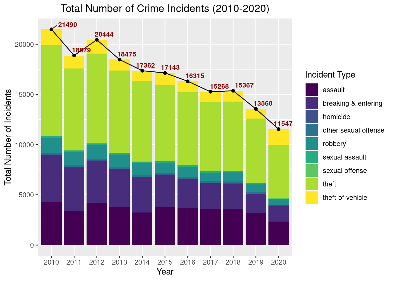
In this part, we create a image to show the change in the total number of crime incidents from 2010 to 2020 and also use distinct colors to mark out different type of crimes.
crime_pre_drop_geo <- st_set_geometry(crime_pre, NULL)

crime_by_year <- count(crime_pre_drop_geo, incident_year) %>%
  arrange(incident_year)

crime_by_year_type <- count(crime_pre_drop_geo, incident_year, parent_incident_type) %>%
  arrange(incident_year)

ggplot() +
  geom_col(data=crime_by_year_type,
           mapping=aes(incident_year, n,
                       fill=parent_incident_type,
                       group = 1)) +
  geom_line(data=crime_by_year, aes(incident_year, n, group = 1)) +
  geom_point(data=crime_by_year, aes(incident_year, n, group = 1)) +
  geom_text_repel(data=crime_by_year, aes(incident_year, n, group = 1, label=n),
                  size=3, fontface="bold", color="darkred",
                  hjust = 0.65, vjust = 0.6) +
  labs(title = "Total Number of Crime Incidents (2010-2020)",
       x = "Year",
       y = "Total Number of Incidents") +
  theme(plot.title = element_text(hjust = 0.5), ) +
  scale_fill_viridis(discrete=TRUE, name="Incident Type")
From the plot above, obviously, it demonstrates that the number of crime incidents has been decreasing through the period of time.
4.1.2 Number of Crime Incidents by Hour
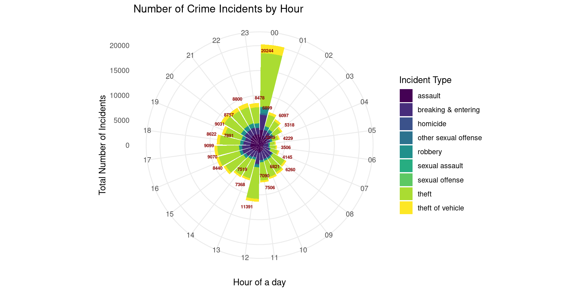
In this part, we attempt to figure out whether there exists a specific period of time that witnesses most crime incidents in a day.
crime_by_hour <- count(crime_pre_drop_geo, incident_hour) %>%
  arrange(incident_hour)

crime_by_hour_type <- count(crime_pre_drop_geo, incident_hour, parent_incident_type) %>%
  arrange(incident_hour)

ggplot() +
  geom_col(data=crime_by_hour_type,
           mapping=aes(incident_hour, n,
                       fill=parent_incident_type,
                       group = 1)) +
  coord_polar(theta="x") +
  geom_text_repel(data=crime_by_hour,
                  aes(incident_hour, n, group = 1, label=n),
                  size=2, fontface="bold",
                  color="darkred") +
  labs(title = "Number of Crime Incidents by Hour",
       x = "Hour of a day",
       y = "Total Number of Incidents") +
  scale_fill_viridis(discrete=TRUE, name="Incident Type") +
  theme(plot.title = element_text(hjust = 0.5)) +
  theme_minimal()
Apparently, as the plot above shows, most crimes are committed in the middle of the night.
4.1.3 Change in the ratios of the types of crime incidents (2010-2020)
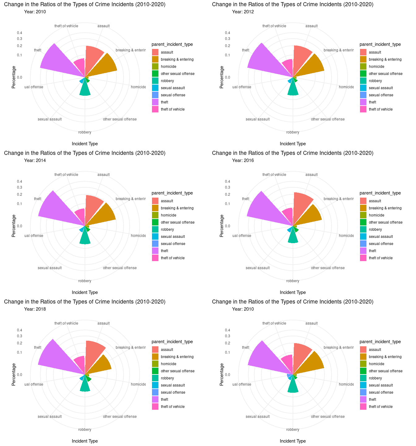
In this part, we explore more about the change in the types of the committed crimes over the 10-year period.
# Firstly, we calculate the ratio (number of crimes of one type in a year / total number of crimes in that year).
crime_by_year_type_ratio <- crime_by_year_type %>%
  group_by(incident_year) %>%
  mutate(percentage=n/sum(n))

# Secondly, we do plotting.
anim <- ggplot(crime_by_year_type_ratio,
               aes(parent_incident_type, percentage, fill=parent_incident_type)) +
  geom_col() +
  coord_polar(theta="x") +
  scale_y_sqrt() +
  theme_minimal() +
  labs(x = "Incident Type", y = "Percentage") +
  theme(plot.title = element_text(hjust = 0.5)) +
  transition_states(as.numeric(incident_year),
                    transition_length=5,
                    state_length=1) +
  ease_aes('linear') +
  ggtitle('Change in the Ratios of the Types of Crime Incidents (2010-2020)',
          subtitle = 'Year: {closest_state}')
animate(anim, renderer = magick_renderer(loop=TRUE))
From the dynamic plot, we notice the three leading types of crime are theft, assault, and breaking&entering. The overall fluctuation of the ratios throughout the 10-year time period is not drastic. However, there is still some shift in terms of two types of crime, namely, assault and breaking&entering.
4.1.4 Map of the Spatial distribution of the crime incident points (2019)
In this part, we create an interactive map showing the spatial distribution of crime incidents in 2019.
# Filter the data for the year of 2019
crime_2019 <- crime_pre %>%
  filter(incident_year=="2019")

# transform the the layers' projection to fit the coordinate system of leaflet map
crime_2019 <- st_transform(crime_2019, '+proj=longlat +datum=WGS84')
Buffalo_CBG <- st_transform(Buffalo_CBG, '+proj=longlat +datum=WGS84')
leaflet(crime_2019) %>%
addTiles() %>% # Add default OpenStreetMap map tiles
addCircleMarkers(radius = 1,
clusterOptions = markerClusterOptions(),
popup = paste0("Crime Type: ", crime_2019$parent_incident_type,
"<br>",
"Date & Time: ", crime_2019$incident_datetime),
popupOptions = popupOptions(closeButton=FALSE, closeOnClick=TRUE)) %>%
addPolygons(data = Buffalo_CBG$geometry,
color = "black",
weight = 0.5)Intuitively, from the map, we are aware that most crime incidents happen within or near the central part of Buffalo.
4.1.5 Map of the Spatial distribution of the crime incidents by Census Block Group (2019)
In this part, we count the number of crime incidents in each Census Block Group and display the map.
# Count by CBGs
crime_2019_count_by_CBG <- crime_2019 %>%
  st_set_geometry(NULL) %>%
  group_by(geoid10) %>%
  summarize(counts = n()) %>%
  # Join the counts to Buffalo_CBG
  right_join(Buffalo_CBG, by = "geoid10")

crime_2019_count_by_CBG <-
  st_set_geometry(crime_2019_count_by_CBG, crime_2019_count_by_CBG$geometry)
pal <- colorNumeric(c('#edf8fb','#b3cde3','#8c96c6','#8856a7','#810f7c'),
crime_2019_count_by_CBG$counts)
leaflet() %>%
addTiles() %>% # Add default OpenStreetMap map tiles
addPolygons(data = crime_2019_count_by_CBG$geometry,
color = "black",
weight = 0.5,
popup = paste0("Number of Incidents: ", crime_2019_count_by_CBG$counts),
fillColor = pal(crime_2019_count_by_CBG$counts),
fillOpacity = 0.8,
highlightOptions = highlightOptions(color = "black", weight = 3)) %>%
addLegend(pal = pal,
values = crime_2019_count_by_CBG$counts,
opacity = 1)4.2 Correlation Between Crime Incidents and Sociodemographic Characteristics
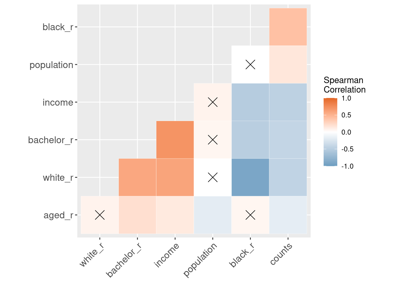
In this part, we explore the correlation between recorded crime incidents and sociodemographic characteristics in the same areas, taking the year of 2019 as an example.
# join the preprocessed demographic data with the crime data of 2019
Buffalo_demo_crime <- Buffalo_demo %>%
  st_set_geometry(NULL) %>%
  inner_join(crime_2019_count_by_CBG, by='geoid10') %>%
  dplyr::select(black_r, white_r, aged_r,
                bachelor_r, income, population,
                counts) %>%
  # There are some missing values in the data frame
  drop_na()
# Calculate the correlation matrix
corr <- cor(Buffalo_demo_crime, method="spearman")
# Calculate the correlation p-values
pmat <- cor_pmat(Buffalo_demo_crime)
# Plot the correlation matrix
ggcorrplot(corr,
hc.order = TRUE,
type = "lower",
outline.color = "white",
colors = c("#6D9EC1", "white", "#E46726"),
ggtheme = ggplot2::theme_gray,
p.mat = pmat,
legend.title = "Spearman\nCorrelation")
The plot of Spearman’s correlation matrix illustrate the potential relationship between crimes and sociodemographic attributes. We find out that the number of crimes is positively correlated with the percentage of black population in a CBG, while the correlations with median household income, percentage of white population, and percentage of reported bachelor’s degree are somewhat negative. There exists little correlation between crimes and total population as well as the elderly population.
5 Conclusion
This project explores the pattern of recorded crime incidents in both time and space dimensions, and also evaluate the correlation between crimes and sociodemographic attributes. The total number of crime incidents has been decreasing from 2010 to 2020. Most crimes are committed in the middle of the night. The overall fluctuation of the ratios of different types of crimes throughout the 10-year time period is not drastic. Spatially, most crime incidents happen within or near the central part of Buffalo. The number of crimes in each CBG is positively correlated with the percentage of black population within a CBG, while the correlations with median household income, percentage of white population, and percentage of reported bachelor’s degree are somewhat negative. There exists little correlation between crimes and total population as well as the elderly population. Base on the results, suggestions are that nighttime security guarantee should be attached more attention to, and that central area of the City of Buffalo, NY needs higher level of public security management.
6 References
- Aksoy, E., 2017. Geography of Crime and Its Relation to Location: The City of Balıkesir (Turkey). IOP Conf. Ser.: Mater. Sci. Eng. 245, 072012. https://doi.org/10.1088/1757-899X/245/7/072012
- Bringing Geography to the Practice of Analyzing Crime Through Technology [WWW Document], n.d. . Office of Justice Programs. URL https://www.ojp.gov/library/publications/bringing-geography-practice-analyzing-crime-through-technology (accessed 11.29.21).
- Butorac, K., 2017. Geography of Crime and Geographic Information Systems. JFSCI 2. https://doi.org/10.19080/JFSCI.2017.02.555591
- Geographic profiling, 2021. . Wikipedia.
- Kaplan, J., n.d. 12 Exploratory data analysis | Crime by the Numbers: A Criminologist’s Guide to R.
- LeBeau, J.L., Leitner, M., 2011. Introduction: Progress in Research on the Geography of Crime. The Professional Geographer 63, 161–173. https://doi.org/10.1080/00330124.2010.547147
- Owusu, G., Frimpong, L., 2020. Crime Geography.
- Understanding Crime: Analyzing the Geography of Crime | Esri Press [WWW Document], n.d. URL 1. https://www.esri.com/en-us/esri-press/browse/understanding-crime-analyzing-the-geography-of-crime (accessed 11.29.21).